e2iminfo.py -H micrograph.mrc

2. Convert MRC to TIF

e2proc2d.py input.mrc output.tif

3. Convert Multiple MRC Files into TIFs

e2proc2d.py *mrc @tif

4. Scale a Map

e2proc3d.py input.hdf output.hdf --clip=140,140,140 --scale=2.8

5. Generate Random Projections of a Map

e2project3d.py map.mrc --outfile=proj.mrcs --orientgen rand:n=10:phitoo=1:trans=4

6. Low-Pass Filter a Map

e2proc3d.py input.mrc output.mrc --process filter.fourier:curres=3.5:targetres=7:dampamp=1:randomizephase=0

7. Sharpen a Map

e2proc3d.py input.mrc output.mrc --process filter.autosharpening:cref=1:mapres=2.5:lpfile=fsc.txt.fit

8. Calculate Structure Factor Curve of a Map

e2proc3d.py input.mrc output.mrc --calcsf output_sf.txt

9. Match Structure Factor Curve to Another Curve

e2proc3d.py input.mrc output.mrc --apix 1.08 --setsf sf.txt

10. Match Filtering Level of Another Map

e2proc3d.py input.mrc output.mrc --apix 1.08 --matchto other.mrc

11. Generate Random 2D Projections from a 3D Map

e2project3d.py map.mrc --outfile=projections.mrcs --orientgen random:n=1000:phitoo=1:inc_mirror=1:trans=10

12. Rotate a Map

e2proc3d.py input.mrc output.mrc --rot az,alt,phi
e2proc3d.py input.mrc output.mrc --rotspin n1,n2,n3,angle

13. Rotate Octahedral Map from 4-Fold View to 3-Fold View

e2proc3d.py input.mrc output.mrc --oct4fto3f
e2proc3d.py input.mrc output.mrc --rot 45,54.7356,0

14. Flip Handedness of a 3D Map

e2proc3d.py input.mrc output.mrc --process xform.flip:axis=o

15. Y-Flip a 3D Reference

e2proc3d.py input.mrc output.mrc --process xform.flip:axis=y

16. Apply Mask to a Map

e2proc3d.py input.mrc output.mrc --process mask.file:file=mask.mrc

17. Apply Cylindric Mask to a Map

e2proc3d.py input.mrc output.mrc --process mask.cylinder3d:innerradius=10A:outerradius=20A:length=60A:masksoft=10A

18. Simulate a Cylinder

e2proc3d.py :96:96:96:1 output.mrc --apix 1 --process mask.cylinder3d:innerradius=10A:outerradius=20A:length=60A:masksoft=10A

19. Simulate a Spherical Mask with RELION

relion_mask_create --denovo --box_size 256 --inner_radius 0 --outer_radius 50 --angpix 1.6 --o mask.mrc

20. Make a Mask Based on Threshold

e2proc3d.py input.mrc output.mrc --process mask.auto3d:nshells=5:nshellsgauss=5:thresh=3

21. Refine and Apply Helical Symmetry

e2proc3d.py input.mrc ouput.mrc --process xform.helical:apix=1.1:az0=22:z0=37.2:cdsym=c6:verbose=1:rstep=1

22. Apply Helical Symmetry Without Refinement

e2proc3d.py input.mrc ouput.mrc --process xform.helical:apix=1.1:az0=22:z0=37.2:cdsym=c6:verbose=1

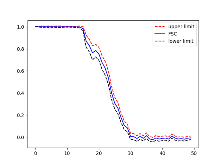
Fourier Shell Correlation (FSC) is the standard method used in the cryo-electron microscopy (cryo-EM) field to estimate the resolution of reconstructed 3D maps, serving as a key indicator of overall map quality. FSC is computed as the cross-correlation coefficient between two independently reconstructed “half maps” as a function of spatial frequency. At each resolution shell, FSC quantifies how well the two maps agree, with higher values indicating better reproducibility and signal.

However, a single FSC value per shell assumes uniformity in signal quality across all voxels within that shell. In practice, this assumption oversimplifies the reality: voxel intensities vary substantially across different spatial locations, even within the same frequency band. This spatial heterogeneity can arise from anisotropic sampling, preferred particle orientations, or local disorder in the structure.

To better capture these local variations, this web application computes FSC not just as an average, but includes statistical confidence intervals around each FSC value. This web app allows you to visualize confidence intervals around the FSC values using three different statistical approaches. You can select your preferred method from the dropdown menu:

1. Fisher Z-Transform Method (Default)

This approach assumes the Fisher z-transformed FSC values follow a normal distribution, allowing us to compute analytical confidence bounds. Formula:

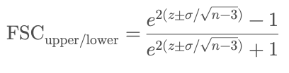
Where:

z = 0.5 × log((1 + FSC) / (1 - FSC)) is the Fisher z-transform of the FSC
n is the number of voxels in the resolution shell
σ (sigma) is a user-defined z-score (e.g., 1.96 for 95% confidence, 3 for 99.7%)
By allowing you to set the sigma value, this app gives you flexible control over the statistical stringency of the FSC envelope, helping you better interpret the reliability of FSC-based resolution estimates.

2. Bootstrap Method

This non-parametric approach resamples voxel pairs within each shell to build a distribution of FSC values. Confidence bounds are calculated from percentiles of this distribution.

• You can adjust the number of bootstrap samples.
• The bounds are based on the 2.5th and 97.5th percentiles by default (95% CI).

3. Variance-Based Method

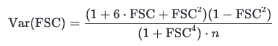
This method estimates FSC uncertainty analytically using a published variance formula that accounts for the number of voxels and the observed FSC value. Confidence bounds are derived as:

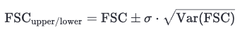
Where Var(FSC) is computed using:

frequency = shell_index / (box_size * apix)  # spatial frequency in 1/Å
resolution = 1 / frequency

Click me to try

Example FSC error bar for EMPIAR 10084 Cryo-EM structure of haemoglobin at 3.2 Å determined with the Volta phase plate

📚 References

• Penczek PA. Resolution measures in molecular electron microscopy. Methods Enzymol. 2010; 482:73–100
  PMID: 20888958 | PMCID: PMC3165049

• Cardone G, Heymann JB, Steven AC. One number does not fit all: mapping local variations in resolution in cryo-EM reconstructions. J Struct Biol. 2013; 184(2):226–236
  PMID: 23954653 | PMCID: PMC3837392

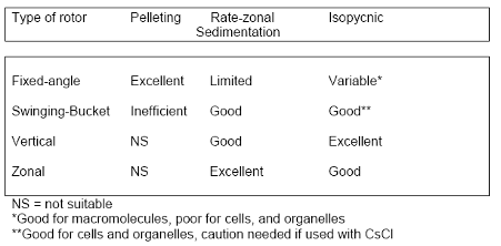
Density gradient centrifugation can be further divided into isopycnic centrifugation and rate-zonal centrifugation.

Isopycnic centrifugation separates particles only based on their buoyant density. It uses a continuous density gradient, which can be either preformed or self-forming (e.g., using CsCl or OptiPrep). In self-forming gradients, the sample is mixed with the gradient material, and the gradient forms during centrifugation. This process typically requires long run times—often overnight—to allow the gradient and particle separation to equilibrate.

Rate-zonal centrifugation separates particles based on their size and sedimentation rate. It often uses a stepwise gradient—a series of discrete layers with increasing density (e.g., 10%, 20%, 30%, 40%). The sample is layered on top of the lightest density layer. This method is widely used for virus purification and typically requires shorter centrifugation times (e.g., one to two hours). However, if spun too long, all particles may eventually pellet, reducing separation resolution.

Sometimes one has to run isopycnic and rate-zonal centrifugation in tandem to enhance purity.

Differential centrifugation or pelleting

• Denser particles are pelleted faster than less dense particles
• Larger particles pellet faster than smaller ones
• Symmetrical particles pellet faster than asymmetrical ones
• Separation is not clean:
  • The g-force used to pellet large particles from the top will also pellet small particles from the bottom

Desnsity gradient centrifugation

Isopycnic Centrifugation (Density Gradient Centrifugation, DCC)

• Separates by density
• Can be carried out in all types of rotors
• Requires longer run times

Preformed Gradient

• Sample volume should be smaller than the gradient volume

Self-Forming Gradient

• Sample is homogeneously mixed with a self-forming gradient (e.g., CsCl or OptiPrep)
• Uses solid gradient material or high-concentration gradient solution
• Centrifuge time is longer than with preformed gradients
• Vertical or near-vertical rotors are preferred
  - Swinging-bucket rotors, which have longer sedimentation paths, are rarely used for self-forming gradients

Criteria for Successful Isopycnic Separation

• Density of the sample particles must fall within the gradient range
• Any gradient length is acceptable
• Run time must be sufficient for particles to band at their isopycnic point
• Excessive run time has no adverse effect

Rate-Zonal Centrifugation

• Separates by sedimentation rates
• Often used for viral purification or characterization
• Initial sample volume should be small
• If run too long, all particles will pellet at the bottom

Rotor Type

• Swinging bucket rotors
• 

⚠️ Care must be taken to avoid “point loads” caused by spinning CsCl or other dense gradient materials that can precipitate.

Centrifugation Time Calculation

The centrifugation time is given by:

The k factor is a measure of the pelleting efficiency of the rotor.

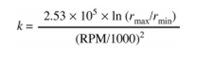
As the k factor decreases, rotor efficiency increases.

Biochem. J. (1976) 159, 259-265

Where:

• t = Centrifugation time
• k = Rotor k-factor (a measure of the pelleting efficiency of the rotor)
  • As the k-factor decreases, rotor efficiency increases
• s’ = Sedimentation coefficient of the particle in a particular gradient at 20°C (in Svedberg units, s)
• ρp = Density of the particle (g/cm³)
• ρ = Density of the gradient (g/cm³)
• ρ₂₀,w = Density of water at 20°C (g/cm³)
• S₂₀,w = Sedimentation coefficient of the particle in water at 20°C (Svedberg units, s)
  • 1 Svedberg (S) = 10⁻¹³ seconds

Example

At 4°C in 20% sucrose, the sedimentation coefficient of Tulane virus:

• s’ = 41.87 S
• Rotor: SW55 Ti, 45,000 rpm
• k-factor = 72.4

Calculation: \(t = \frac{k}{s'} = \frac{72.4}{41.87} \approx 1.73\ \text{h} \approx 2\ \text{hours}\) —

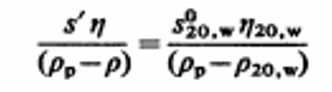
Note: The sedimentation coefficient is influenced by the viscosity and density of the sucrose solution. Viscosity is dependent on both concentration and temperature.

Check out the Practical Techniques for Centrifugal Separations for more details.

The tutorial commands result in error messages.

git clone https://github.com/czimaginginstitute/AreTomo3.git
cd AreTomo3
make -f makefile11 CUDAHOME=/usr/local/cuda \
     CXXFLAGS="-I/usr/local/cuda/include" \
     LDFLAGS="-L/usr/local/cuda/lib64"

a. Transfer Shuttle Drying

• Dry the Transfer Shuttle on the Leica Cryo Tool Dryer (CTD) for at least 20 minutes before use to reduce contamination.

b. Cryo Stage Heating

• Run stage heating for 30 minutes at 60°C:
  • Do not connect the LN₂ hose.
  • Lift the objective to the uppermost position (fully retracted).

2. Power On Sequence

a. Microscope

• Turn on the microscope, the control panel and the pump.
• Turn on the camera.

b. Laser

• Important: Turn on the front switch of the laser before the back switch.
  • Otherwise, the laser will not power on.

3. Launch Imaging Software

• Start LAS X software.

4. Initialize Motorized Stage

• Click Initialize Stage.
• ⚠️ Do not block the stage — allow it to move freely during initialization.

5. Select Imaging Mode

• Navigate to:
  MatrixScreener → Matrix MAPS + CLEM

6. Fill Liquid Nitrogen (LN₂)

• Fill LN₂ into the storage tank.
• ⚠️ Do not fill all the way to the top:
  • LN₂ may spill when inserting the heat exchanger.

7. Connect Cryo Hose to Pump and Stage

a. Start the Pump

• Press COOL to start.

b. Wait for Purge

• Wait until the hose is purging nitrogen gas.

c. Connect Hose to Cryo Stage

• Insert the hose into the cryo stage.
• Lock the hose in place:
  • Push the locking screw toward the hose while tightening.
  • ⚠️ If not pushed first, the hose may be pulled out easily and won’t seal properly.
    • Moisture may enter and condense, blocking the view.

8. Wait for Stage Cool Down

• When temperature reaches -195°C, wait another 15 minutes before loading the sample.

9. Cool Down the Transfer Shuttle

a. Setup

• Ensure the transfer shuttle shutter is closed.

b. Insert Cartridge

• Place an empty cartridge into the loading position.
• Close the slider.
• Turn the rod to the open-O position.
• Cover the cartridge with the shielding.

c. Fill LN₂

• Cover the transfer shuttle with its lid.
• Open the rotatable opening.
• Fill LN₂ inside the shuttle.
  • ⚠️ Do not overfill — avoid pouring over the rod.
  • Otherwise, the rod may freeze and become immobile.
• The shuttle is fully cooled when the LN₂ stops boiling inside.

10. Load AutoGrids into Cartridge

• Proceed with loading autogrids into the pre-cooled cartridge.

11. Load Grid into Microscope

a. Ensure Lens Is Up

• ⚠️ Objective lens must be lifted to avoid damage from the shuttle.

b. Stage Access

• Open the stage slider.

c. Insert Transfer Rod

• Insert the transfer rod fully.
• Rotate to Open position to release the cartridge.
  • ⚠️ Must insert all the way to the end.
  • Otherwise, you won’t be able to focus on the grid.

d. Retract Rod

• Pull the rod back.
  • The cartridge should remain in the stage.

e. Clean Up Shuttle

• Remove the transfer shuttle from the stage.
• Pour out any remaining LN₂.
• Place it on the Cryo Tool Dryer (CTD) for baking out.

12. Imaging Procedure

a. Load Experiment

• Open LAS X and load your experiment.

b. Move to Left Grid

• In the MatrixScreener window:
  • Right-click the left grid.
  • Select “Move stage to left grid center”.

c. Autofocus

• Run Auto Focus.
• ⚠️ If autofocus fails, adjust manually until sharp.

d. Spiral Scan

• Run the Spiral Scan to locate good regions for imaging.

e. Focus Map Setup

• Select a circular imaging area.
• Click on several points within the circle to define a focus map.
• Click Start Focus Map to collect Z positions.

f. Mosaic Scan

• Enable 4 channels.
• Adjust the Z-stack range according to your sample thickness.
• Click Run Matrix to begin automated imaging.

g. Export Data

• After acquisition is finished, export data files for downstream analysis.

13. Finishing Up

a. Close Software

• Exit the LAS X software and any other imaging applications.

b. Retrieve Grids

• Lift the objective lens to its uppermost position.
• Retrieve the cryo grids from the stage.

c. Heat the Stage

• On the temperature control box, press “Heat”.
• Wait until the stage heats to 60°C.

⚠️ Do not remove the hose before the temperature reaches 60°C.
Removing the hose prematurely can cause damage due to freezing.

d. Disconnect the Cryo System

• Once the stage is at 60°C:
  • Remove the LN₂ hose.
  • Remove the pump from the LN₂ tank.

e. Return Grid Boxes

• Place the used grid boxes back into the LN₂ storage tank for long-term storage.

• Write down chamber pressure.
• Fill liquid nitrogen to the tank.
• Cool down the heat exchanger.
• Set N₂ gas flow rate to 180 mg/s.

Step 2: Chamber Check

• Check if there is any sample in the chamber.

Step 3: Grid Loading

• Wait 1 hour after cooling down, then load grids.

Step 4: System Wake-up and Beam Alignment

• Wake up the system.
• Turn Beam On.
• Perform 180° scan rotation for both holders.
• After rotation, ensure the slot is positioned at the bottom of the grid.

Step 5: Grid 1 Mapping Preparation

• Navigate to lowest magnification.
• Press F6 to enable live view.
• Switch to higher magnification.
• Perform coarse focus.
• At 2000x, do fine focus.
• Perform Sigma X and Y alignment.

Step 6: Z-Height Calibration

• In live mode, select Link Z to Forward.

Step 7: Project Setup in MAPS

• Open MAPS.
• Create a new project.
• Change save location to:
  \\AS-SPC\SharedData\Chen\20241106

Step 8: Grid 1 Pre-GIS Mapping

• Go to lowest magnification.
• Take a snapshot.
• Add tiles.
• Rename to “Grid1-preGIS”.
• Click Run.

⚠️ Repeat Steps 5–8 for Grid 2.

Step 9: Cryo-CLEM Data Integration

• Import cryo-CLEM data.
• Align the data.
• Add lamella positions.

Step 10: Sputter Coating Preparation

• Increase N₂ gas flow to 210 mg/s.
• Perform Sputter coating using Setting 1 for 15 seconds.

Step 11: GIS Deposition on Grid 1

• Apply GIS to Grid 1 for 10 seconds.

  ⚠️ Do not exceed 10 seconds. A thick GIS layer will hinder milling efficiency.

Step 12: Post-GIS Coating

• Perform Sputter coating again.
• Reset N₂ gas flow to 180 mg/s.

Step 13: High-Resolution Imaging (Grid 1)

• In XT-UI, take a high-resolution image.
• Save as: Grid1_afterGIS-XXX.tif.

Step 14: AutoTEM Setup

• Open AutoTEM.
• Change project name.
• Do not change save location (keep as D:\AuToTEM Cryo\Projects).

Step 15: (intentionally left blank for future use)

Step 16: Lamella Preparation

• Start lamella preparation.
• Manually adjust lamella placement.
• Proceed with milling and thinning step-wise.

Step 17: Manual Fine Polishing

1. In AutoTEM, select the lamella → Right click → Go to lamella position.
2. Increase tilt angle by +0.5° (e.g., T = 16.5 if stage = 16°).
3. Create a rectangle milling pattern, set direction: top to bottom.
4. Adjust brightness and contrast using a pattern at the side.
5. Position milling pattern on top of the lamella.
6. Start milling with 30 pA ion beam.
7. Use image shift Y to gently move the lamella into the milling pattern.
8. Check lamella thickness with SEM view (2 kV).

   A thin lamella should appear black in SEM.

Step 18: Documentation

• In MAPS:
  File → Save screenshot as → Save grid image with lamella positions.
• In XT-UI:
  • Take SEM and FIB images after focus adjustment.
  • Use the finest photo button.
  • Save images as:
    • L2_i.tif
    • L2_s_2kV.tif
    • L2_1200x_2kV.tif (for LM correlation)
• Go to lowest magnification → Take full grid image with SEM.
• Copy entire data folder to the lab server.

Step 19: Shutdown Procedure

• Put the system to Sleep.

  ⚠️ This is important to prevent ion beam waste.

• Reset N₂ gas flow rate to 12 mg/s.

Clone the GitHub repository and follow the instructions in the README to install dependencies and set up the Python environment:

Step 2: Select a Specific GPU

To specify which GPU to use, prepend your MemBrain command with the CUDA_VISIBLE_DEVICES environment variable. This variable tells PyTorch which GPU(s) are visible to the program. You can run multiple MemBrain commands in parallel on different GPUs to process several tomograms simultaneously.

CUDA_VISIBLE_DEVICES=1 membrain segment --tomogram-path lamella4_ts_001_full_rec.mrc --ckpt-path /home/csun/Membrain-model/MemBrain_seg_v10_alpha.ckpt --store-connected-components